Lending Club Loan Analysis
Maximizing Investment Returns using Machine Learning
By: Saleem Khan

Photo by Alexander Mils from Pexels
Key Takeaways
- 7.41%
- The percent of overall bad loans within the Lending Club portfolio in 2018.
- 22.89%
- The actual percent of bad loans when removing “current” loans which have not fully paid out yet.
- Small Businesses
- Tend to default the most when examining the most frequent borrowers.
- Machine Learning
- Can be used to create a portfolio which beats the average total return for randomly chosen loans.
Background
Founded in 2006, Lending Club is the world’s largest peer-to-peer lender. They disrupted the traditional bank-based personal lending market by allowing retail investors to lend directly to individuals wanting to borrow. The Lending Club loan pool has grown steadily since its founding. In the last 3 years the platform originated nearly $18B in new loans.
Problem Statement
- What is the actual default rate for Lending Club loans? I wanted to take a deeper dive into the actual default rates within Lending Club so investors can make a more informed decision about their risks.
- Who tends to default the most? I wanted to see whether risk was pooled within a certain borrower type or loan purpose so we can make sure to have a diversified portfolio.
- Is it possible to use a classification model to determine, with high accuracy, whether a loan will default? I wanted to use a classification model to determine whether we can beat the average total return for a randomly selected pool of loans.
Exploratory Data Analysis
Lending Club is quite unique in that it offers all members access to loan data going back to their inception. If you visit the Lending Club Statistics page you will be able to download data and statistics going back to 2007. However, for the purpose of this exercise I decided to look at data for 2018 only.
After downloading the dataset one of the first things you notice is how verbose it is. There are nearly 150 unique columns of information ranging from the basics (e.g. loan amount, debt-to-income and interest rate) through to detailed attributes such as the number of derogatory public records and tax liens. This makes the dataset incredibly rich and full of potential predictive power.
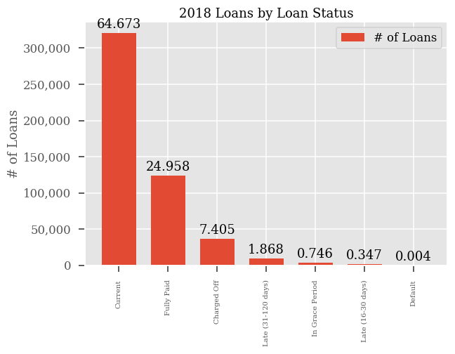
A majority of the loans within the 2018 dataset are “current”. Lending Club distinguishes between seven distinct loan statuses. However, for my goal of generating a machine learning model there are really only two statuses that I care about: whether a loan turned out to be a good loan (i.e. fully paid) or a bad loan (i.e. default or charged off). These two states will be my dependent variable (i.e. the output I’m trying to predict) in my machine learning model. One thing to note here also is that I am not including any loans that are late or in a grace period. As you can see from the chart above these statuses don’t occur very often and would not be statistically relevant since we would not have outcomes that can be included in our dependent variable.
What is the overall default rate for Lending Club loans?
This is a bit of a perspective-based question. It really depends on whether you only want to look at loans where there is an outcome (e.g. a binary answer of whether the loan defaulted or not) or whether you wanted to look at the entire Lending Club portfolio en masse. The table below shows the overall statistics.
| Overall | Count | Percent |
|---|---|---|
| Good Loans | 458,551 | 92.59% |
| Bad Loans | 36,691 | 7.41% |
However, if we change the perspective here and remove all current or late loans (i.e. loans where we have not outcome yet) then we get a very different picture:
| Ex. Current | Count | Percent |
|---|---|---|
| Good Loans | 123,603 | 77.11% |
| Bad Loans | 36,691 | 22.89% |
Our default rate almost triples when we remove current loans. The next logical view is to look at the data from the perspective of risk ratings. Lending Club assigns a letter grade to each loan as part of an upfront due-diligence process where a borrower’s ability to repay is analyzed. Lending Club collects everything from FICO scores through to revolving credit amounts. They assign letter grades in the range from A-G (A being the highest grade). Here is the occurrence of defaults by letter grade:
| Grade | Default Rate |
|---|---|
| A | 2.37% |
| B | 5.64% |
| C | 9.28% |
| D | 13.63% |
| E | 17.84% |
| F | 23.87% |
| G | 28.02% |
Who tends to default the most?
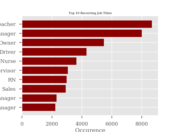
There is a wealth of information in the Lending Club data however personally identifiable information (PII) is not available. In lieu, Lending Club provides distinct job titles as reported by the borrowers within the platform. When doing a basic search of the most commonly occurring job titles, we find the following:
| Job Title | Frequency |
|---|---|
| Teacher | 9982 |
| Manager | 9547 |
| Registered Nurse | 8125 |
| Owner | 7426 |
| Driver | 5421 |
| Supervisor | 3799 |
| Sales | 3683 |
| Office Manager | 3017 |
| Truck Driver | 2905 |
| Project Manager | 2780 |
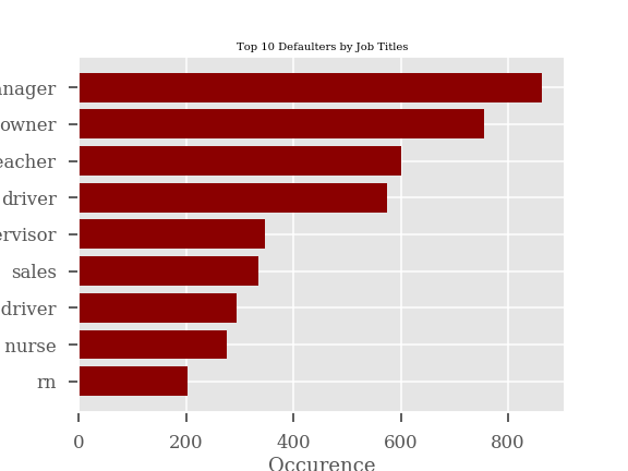
However, when we look at the top 10 job titles by defaulters we see some of the statistics paint a slightly different picture. We see below that the top defaulters are managers and owners. After browsing some these loans and looking at the loan purpose and description it looks like owners and managers are most likely individuals running small businesses. These borrowers account for almost 2x more defaults than the next most frequent profession.
Machine Learning
Now we will examine whether we can create a generalized machine learning model that is able to predict whether a loan will default or not. In order to conduct this analysis, we first need to look at a correlation heatmap in order to get a sense of how much our independent variables (or features) impact our dependent variable. As mentioned earlier our dependent variable is a flag which will denote whether a loan defaulted or not and our independent variables will be the 150 columns we received from Lending Club.
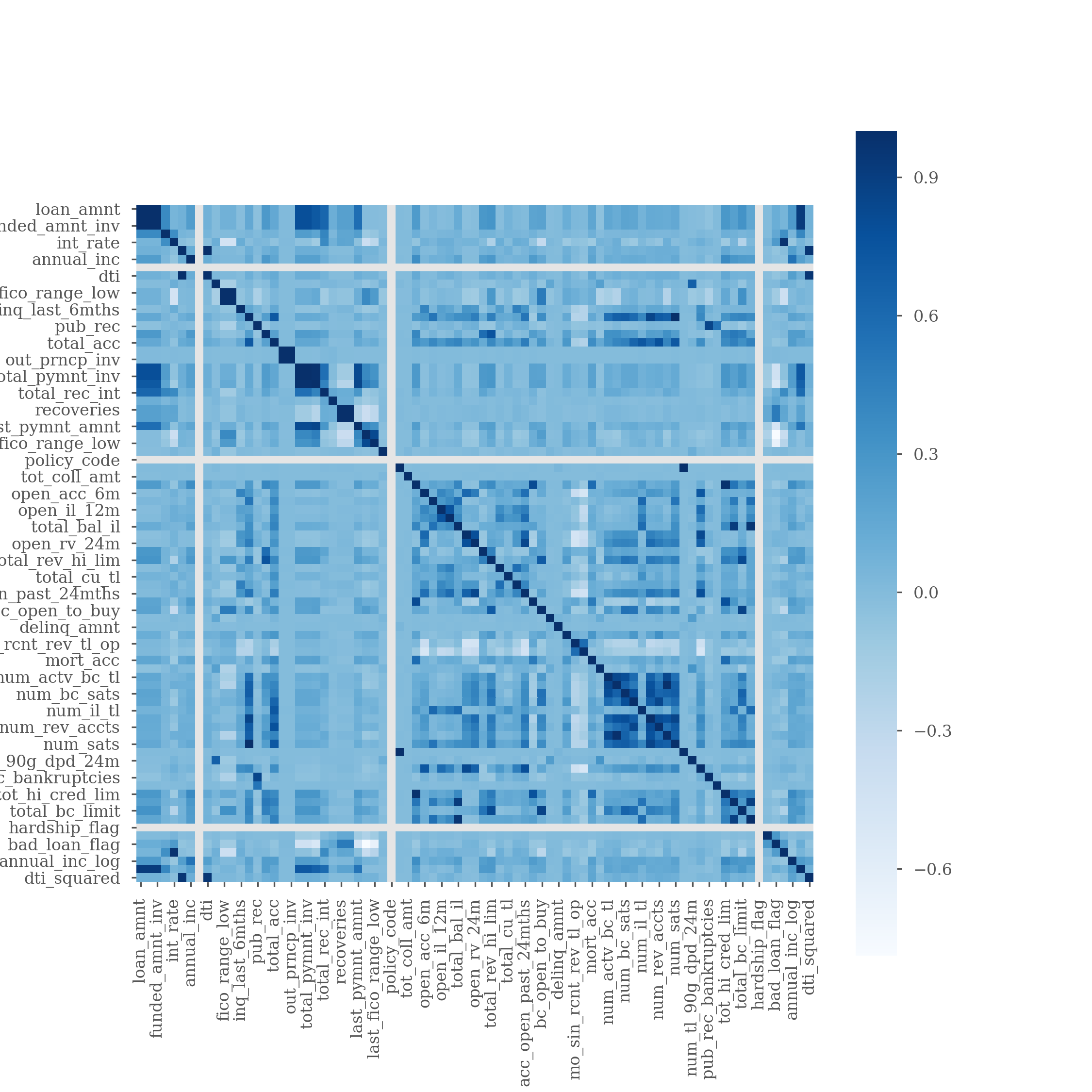
The chart above is quite difficult to read because of the sheer volume of features we have access to. However, the big takeaways are that income, loan amount and interest rates are among the top factors that impact our dependent variable (e.g. bad_loan_flag). Let’s move ahead with this and take a look at creating some baseline models.
Baseline Model
I started with creating some baseline models that were not optimized. I looked at the following:
- Random Forest
- A decision tree based algorithm that examines the relative weights of a series of decision models to predict an outcome.
- Gaussian Naive Bayes
- A basic probabalistic approach to logistic regression.
- KNN (K Nearest Neighbors)
- An approach which looks to cluster outcomes based on Euclidean distance.
- Decision Tree
- A simpler version of Random Forest
- Logistic Regression
- A form of linear regression that creates an S-shaped curve instead of a straight line in order to classify observations.
When comparing models there are quite a few metrics we can analyze. There is accuracy, precision, recall, F1 and ROC/AUC. Since we have a highly imbalanced class here – that is, we have very few occurrences of defaults as opposed to good loans – our best metric will be the ROC/AUC metric. Without getting into too much detail: accuracy, precision and recall are not great metrics for imbalanced classes. A high number of false positives (predicted good loans that were actually bad) is an undesirable outcome, because we are trying to optimize for higher returns in our portfolio.
All of the models I analyzed had very similar ROC AUC metrics. AUC is short for the area-under-the-curve and is a plot of comparison between our true positive and false positive rates.
| Classification Model | ROC/AUC |
|---|---|
| Random Forest | 0.54 |
| Gaussian Naive Bayes | 0.54 |
| KNN | 0.53 |
| Decision Tree | 0.54 |
| Logistic Regression | 0.53 |
An ROC/AUC score of 0.50 is essentially a coin flip so our model right now is barely doing better than a coin flip at predicting whether a loan will be good or not. Let’s now start tuning and using some different techniques.
Class Imbalance
Since I have a large imbalance in my target variable I decided to use a technique called random oversampling in order to balance my classes. I went from an imbalance of 3.37 : 1 (good loans to bad loans) to a 1:1 ratio using this technique. Random oversampling just randomly recreates members of the minority class to balance out classes. There are other techniques that I tried as well called random undersampling, ADASYN and SMOTE. Random undersampling as the name implies is the opposite of oversampling and ADASYN and SMOTE essentially create synthetic entries (i.e. made up observations) to mimic the minority class. Once I applied the class balancing techniques, here were my ROC/AUC scores:
| Classification Model | ROC/AUC |
|---|---|
| Random Forest | 0.54 |
| Gaussian Naive Bayes | 0.63 |
| KNN | 0.56 |
| Decision Tree | 0.54 |
| Logistic Regression | 0.64 |
Interestingly most of my scores didn’t change with the exception of GNB and Logistic Regression. I’m not 100% sure why those scores seemed to do better but when I tested these models with a Monte Carlo simulation which simulates a loan portfolio, these models were performing only as well as a random guess so they don’t seem to have much predictive power.
I then tried to optimize the Random Forest approach with a random search optimization. This approach tries to go through random hyperparameter selection until it finds an ideal number of decision trees for our forest. After trying this approach and settling on six decision trees I still had an ROC/AUC of 0.54; barely better than a coin flip.
Time to Pivot
As frustrating as it was going through the above and not coming out with a highly predictive model I decided to push ahead and reframe the problem a bit. I mentioned earlier that there are investment grade and non-investment grade loans in this portfolio. I had a hunch that the investment grade loans were somehow diluting the predictive power within this dataset because the default rates were so low for A, B and C rated loans. I decided to take a closer look at just the non-investment or junk loans to see if I could find any alpha here. Long story short; I did!
Once I removed the investment grade loans and went through the same process above to train a model to this new dataset I started seeing much better metrics. The hero model (or winner) in this second pass was a random forest algorithm which had great scores across the board and an ROC/AUC of 0.75 (way better than a coin flip).
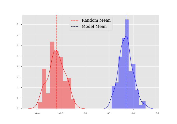
I created a Monte Carlo simulation that visualizes my returns using this approach. The chart below is a visual representation of two loan portfolios. The red represents 100 simulations (or iterations) of a randomly chosen portfolio of 100 loans. The dotted red line represents the mean total return for this portfolio. Notice that the return is actually a -0.25, meaning the average random portfolio would return 25% less than the principal. The blue bars represent loans that were selected using my Random Forest model. You’ll notice that we yielded a positive mean total return of nearly 0.35 (or 35% above the principal) on this portfolio. This is almost a 60% improvement in total returns over a randomly chosen portfolio!
Conclusion
So what were the main features that influenced our outcome variable the most? There should be no surprise here but the top features and their relative weights are below:
| Feature Variable | Weight |
|---|---|
| Interest Rate | 0.49 |
| Annual Income | 0.19 |
| Loan Amount | 0.15 |
| FICO Score | 0.12 |
| Debt-to-income | 0.03 |
Interest rates seem to have a huge impact on whether a loan will default or not. I did a quick query to look at average interest rates by letter grade and the corresponding default rates, here were the results:
| Grade | Average Int. Rate | Default Rate |
|---|---|---|
| A | 7.06% | 2.37% |
| B | 10.86% | 5.64% |
| C | 14.68% | 9.28% |
| D | 19.50% | 13.63% |
| E | 25.22% | 17.84% |
| F | 29.48% | 23.87% |
| G | 30.81% | 28.02% |
Lending Club interest rates can range from 7% for A-graded borrowers all the way up to a whopping 30% for an F-graded borrower. To put that in perspective, a 30% interest rate on a 3 year loan of $10,000 amounts to $5,282 in interest payments. That’s more than 50% of the original loan amount! It’s no wonder that these poorly graded loans not only carry a high interest rate but also have a 30% chance of defaulting.
Final Thoughts
My big learning from this exercise is that creating models is never easy but more importantly I learned that domain knowledge and knowing your data is key. If I had not pivoted to looking at the non-investment grade loans I don’t think I would have been able to find any alpha in this data.
As a follow up for future work here, I will be looking to apply some ensembling techniques (essentially stringing models together to get better predictive power) as well as potentially looking at a much larger sample of the Lending Club data to see if we can find some predictive lift in the investment-grade pool of loans.
Code - All python code for this project can be found in my GitHub respository: GitHub