Classifying The Web

Big Data & Machine Learning for B2B Marketers

By: Saleem Khan

Key Takeaways

• 25.1%
  • The approximate percentage of websites that can be classified as businesses or e-commerce related on the open web.
• 650 Million
  • The number of web pages that are potential businesses that B2B marketers could market to. This number is based on 2.6 billion web pages collected in February of 2020 by a web archive called Common Crawl.
• 11 to 1
  • Based on the above analysis and roughly speaking, for every 11 people in the world there is one business.

Background

In this exercise I will be examining the use of web archive data to produce valuable insights and data assets for Business-to-Business (B2B) marketers. B2B marketers are looking for accurate business information in order to precisely target certain kinds of businesses. There are traditional methods of using directories and business registries but the most up-to-date information on a business can usually be found on its website. Therefore, knowing whether a website is a business website or not is a valuable first step for marketers to have up-to-date and highly accurate information on the audiences they are targeting. In this blog post, I will be walking through the steps required to produce a dataset that can put data scientists on a path to extracting this valuable information for their marketing teams.

Problem Statement

• Is it possible to use data from the web to identify businesses?

  I wanted to develop a machine learning model that can look at the raw text of a web page and determine whether it is a business or not.

Goal

The ultimate goal here is to use a classification model to produce a curated list of business websites that can then be further categorized based on keywords. These further categorizations will, for instance, classify a business as being a bank or a grocery store. One example use-case here would be a company that manufactures cardboard boxes for pizza delivery. This sort of company will mainly sell to pizza parlors. Their marketing team would need an accurate and holistic dataset of pizza parlors in their region or country to effectively market to this audience. This sort of information is key in effective B2B marketing. A final goal would be to pull all relevant contact information such as e-mail, phone and address so marketers can then communicate with each business.

Approach

The approach I will be taking here is threefold:

1) Dataset

Common Crawl is an open repository of web crawl data. This data is refreshed monthly with a history that goes back to 2011. Each month contains nearly 260 terabytes of information. To put this number in perspective, if you were to print out all this monthly information you would have a stack of papers about 16,000 miles tall. That is enough to wrap more than half way around the circumference of the Earth. All of the data in CommonCrawl, from 2011 to the present day, would take you to the moon and back over 6 times!

2) Classification

scikit-learn is a simple and powerful library built on Python’s numpy and pandas frameworks. This library provides great machine learning capabilities. I will be focused on classification models since my goal will be to determine whether a website is a business or not. The model that I develop here will be created on a subset of my data and will eventually be used on a larger dataset of Common Crawl data.

3) Big Data Processing

The last item here is to run my classification model against a random sample of Common Crawl data. Since this is such a large dataset, I will need to use technology that allows me to parallelize the task and work efficiently to extract the classifications I’m looking for. I will be using Apache Spark which is a highly efficient data processing tools that uses Directed Acyclic Graphs (DAG) to process data and stores the output in Resilient Distributed Datasets (RDD). I will also be using the Amazon Web Services (AWS) cloud, specifically AWS Elastic Map Reduce (EMR) and AWS Simple-Storage-Solution (S3) in order to run my Spark job and analyze Common Crawl data.

Step 1 - Dataset

Common Crawl crawls the web and freely provides its archived datasets to the public. Web archives consist of petabytes of data collected since 2011. The archived data comes in three distinct file formats:

1. WARC - this is a web archive file that contains the raw data collected from each web page that was crawled
2. WAT - metadata extracted from a WARC file which shows information like the HTTP request, response and associated metadata (e.g. server type, IP address & cookie information)
3. WET - plain text extracted from the WARC file. This includes the payload of the webpage and some basic metadata like the URI.

Here is a view of an actual WARC file:

Since I will be focusing my analysis on the latest extract of Common Crawl I will be using this link. This referenced file contains the February 2020 WET plain text extract pointers in Amazon S3. The nice thing here is that I do not need to download the full 260 terabytes since AWS hosts Common Crawl data and allows users public read-only access. This wet.paths.gz file contains a gzip listing of paths to the actual crawl data.

Note: I will share my full source code at the end of this post but one thing to note here is that the Common Crawl pointer files do not include the fully-qualified S3 paths. You will need to modify the downloaded wet.paths.gz file by changing an entry like this:

crawl-data/CC-MAIN-2019-35/segments/1566027312025.20/wet/CC-MAIN-20190817203056-20190817225056-00000.warc.wet.gz

to this:

s3://commoncrawl/crawl-data/CC-MAIN-2019-35/segments/1566027312025.20/wet/CC-MAIN-20190817203056-20190817225056-00000.warc.wet.gz

Notice the addition of s3://commoncrawl/ before the path. An easy way to make this change is to download a text editor like Sublime Text and on a Mac hit Cmd + Option + F in order to do a regular expression find and replace of all entries of crawl-data with s3://commoncrawl/crawl-data.

Now the Common Crawl dataset is ready to be processed by my Spark job.

Step 2 - Classification Model

Before I get into the Spark job creation I will need to create a model that can determine whether a webpage is a business or not. I’ve broken this task down into four steps:

1. Training Data
2. Natural Language Processing
3. Modeling
4. Model Selection

Training Data

Note the source code for the discussion below can be found in: BusinessClassifier_Modeling.ipynb

The training data that I will be using will come from the sklearn.fetch_20newsgroups dataset. This dataset is included as part of the scikit-learn library and includes a pre-labeled dataset of raw text that has been classified as being a member of 20 different topics.

The image below shows the pre-labeled topic descriptions and the sklearn topic names. The reason I decided to use this dataset to train my model is:

a. In lieu of going through the laborious task of creating my own pre-labeled dataset of sample articles mapped to topics this dataset is already pre-labeled for me and

b. luckily this dataset actually includes e-commerce or business-related text already. The item highlighted in white below E-Commerce or misc.forsale contains newsgroup comments and articles about businesses.

The fetch_20newsgroupds data set contains 11,314 documents with 130,107 unique words.

Natural Language Processing

The next step is to take all the text in all of my documents and extract the most relevant terms for each topic. I will be using a technique called TF-IDF (Term Frequency multiplied by Inverse Document Frequency). At a high level this approach tries to determine the importance of a word in a document by assigning a relevance score. At a high level, here’s how it works:

a. Term Frequency: the number of times a word appears in a single document divided by the number of words in the document.

b. Inverse Document Frequency: the log of the 11,314 documents in this corpus divided by the number of documents that contain the word being evaluated.

Multiplying these two terms will give me a value for each word in each article that ranges from 0 to <1. The higher the number the more important a word is to a particular article. So for each row of my dataset (i.e. each article) I will have 130,107 features but only a small number will be populated with a TF-IDF score. These scores combined with the unique words are the features that I will be passing into my machine learning model in order to classify an article as being business related or not.

Modeling

Modeling is actually a pretty easy part of this entire exercise. scikit-learn contains models that often take just a few lines to run. I analyzed a few different classification models:

1. Multinomial Naive Bayes: This model is a variation on the basic Naive Bayes model which works by classifying our input record by calculating conditional probabilities for word importance using Bayesian inference. The multinomial part of this model simply allows us to have more than just a binomial (i.e. binary) distribution for our classifier. So for instance, I have 20 categories above that need to be classified. This model will allow us to create a model that separates all 20 categories using conditional probabilities for words.
2. Decision Tree Classifier: Consists of a large number of individual decision trees that operate as an ensemble.
3. Random Forest Classifier: A variation on the Decision Tree algorithm except this approach uses a voting technique to determine which trees are best to use.
4. Linear Support Vector Classifier: Support Vector Machines or in this case Support Vector Classifiers are a type of supervised machine learning model that attempt to find a hyperplane in n-dimensional space that distinctly classifies data points.

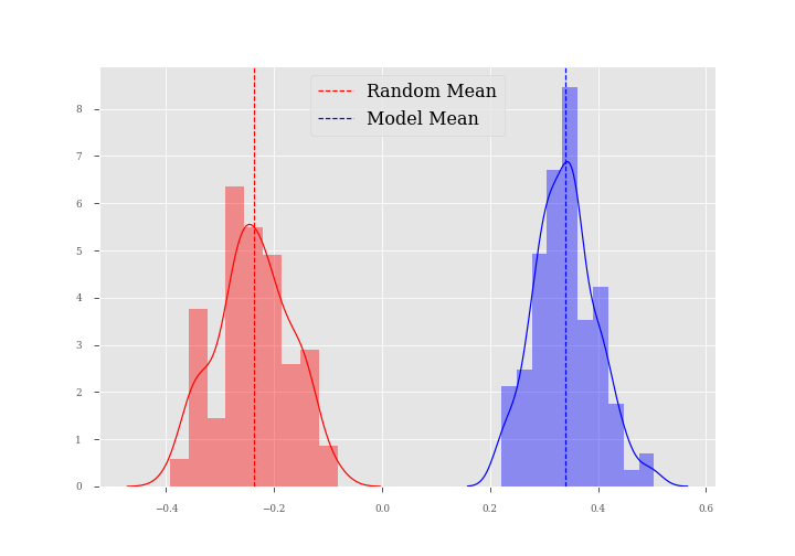
Model Selection

After running these models against my pre-labeled training data and producing a model it was time to use an out-of-sample test dataset that I set aside in order to calculate my model accuracy. After analyzing the model accuracy scores the Linear SVC model came out on top.

In the Linear SVC approach each data point is first plotted in n-dimensional space. Since I have 130k+ features let’s work with a smaller dataset of just a few terms to analyze how Linear SVC works. The image below is a view of random data plotted in two dimensions. Assume the purple dots represent business-related terms like: sell, price and offer and the yellow represents terms used in baseball like: strike, homerun and batter. The x-axis in this case would represent my TF-IDF values and the y would be each word. The clusters would then represent topics like e-commerce and baseball.

What Linear SVC does is it draws a line of best fit with the largest margin possible (also called a support vector, hence the name) which separates categories as being part of one class or the other. This is the core concept of how a support vector classifier works. The image below is a view of this line along with its margin being drawn.

After completing this exercise my model produces pretty high accuracy, precision and recall score as seen below:

However, I can’t merely rely on these metrics. The other way to determine whether my model is accurate or not is to look at the top ten keywords that were associated to each topic. By looking at the table below, specifically the E-commerce topic I can see that commerce-related terms like asking, sell, shipping, offer and sale are showing up. This shows that the model is doing a pretty good job selecting relevant terms for each topic.

Sanity Testing

One final step here is to test my model against some sample data from Common Crawl. I took a few random business-related websites and ran them through my model. The first website below was for a manufacturer in China that my model classified correctly. The second was a business in Cincinnati, Ohio that was selling tickets to a play which was also classified correctly. The last one however was a mobile phone review site which was incorrectly classified as a business. It is expected to get some false positives in a dataset like this but overall the model is doing a pretty good job.

Step 3 - Big Data Processing

Now that I have a model that works and a dataset that is prepped I need to determine an efficient approach to running my model against the Common Crawl data. For the purposes of this exercise I will be taking a 1% random sample of the 260 terabyte Common Crawl file from February 2020. This sample will contain about 2.6 terabytes of information on 25 million web pages. Based on the Central Limit Theorem, this should be a very representative sample of the overall population.

The approach here involves three major technical components:

1. Apache Spark - used to highly parallelize and scale the processing of my data
2. Amazon S3 - used to store and retrieve the Common Crawl web archive data and Spark output
3. Amazon EMR - a cloud-based platform that hosts Spark jobs that run on Hadoop.

After going through all the setup and scripting I attempted to run my Spark job on a 100 node cluster but was rejected because of an Amazom EMR instance limit constraint. I was eventually able to request a limit increase from Amazon support but not in time for this analysis. I was able to run a 4 node Spark cluster for about two days at a cost of $50. This is a relatively cheap price to process such a large amount of information! With my new 100+ instance limit it would take approximately 1.92 hours and about $30 to process this same amount of data; a significant decrease in time and cost!

For more details on the exact steps involved here, please refer to the README.md file in my GitHub repository.

Results

So how is the web categorized? Turns out the web is used to do a lot of business. As a matter of fact, the majority of the web is used for commerce. Almost 25.1% of pages were classified as being business or e-commerce related. Extrapolating this percentage out we get a rough estimate of 650 million web pages within the Common Crawl archive are potentially businesses!

Final Thoughts

A few follow-up items here for future development:

• Business Identification: A follow-up item is to create a custom dataset that contains 100k businesses and non-businesses to train a more updated version of my model. The fetch_20newsgroups dataset is a bit dated and may not capture newer business terminology.
• Business Categorization: Another item here is to classify the businesses identified into distinct types of businesses like banks and grocery stores using both keyword assignment as well as industry classifiers such as SIC, NAICS and NACE codes.
• Business Contact Data: Start to scrape anything resembling an e-mail, phone or address on each web page along with business name.

Code - Thanks for making it this far… all Python code for this project can be found in my GitHub repository: GitHub

Lending Club Loan Analysis

Maximizing Investment Returns using Machine Learning

By: Saleem Khan

_{^{Photo by Alexander Mils from Pexels}}

Key Takeaways

• 7.41%
  • The percent of overall bad loans within the Lending Club portfolio in 2018.
• 22.89%
  • The actual percent of bad loans when removing “current” loans which have not fully paid out yet.
• Small Businesses
  • Tend to default the most when examining the most frequent borrowers.
• Machine Learning
  • Can be used to create a portfolio which beats the average total return for randomly chosen loans.

Background

Founded in 2006, Lending Club is the world’s largest peer-to-peer lender. They disrupted the traditional bank-based personal lending market by allowing retail investors to lend directly to individuals wanting to borrow. The Lending Club loan pool has grown steadily since its founding. In the last 3 years the platform originated nearly $18B in new loans.

Problem Statement

• What is the actual default rate for Lending Club loans? I wanted to take a deeper dive into the actual default rates within Lending Club so investors can make a more informed decision about their risks.
• Who tends to default the most? I wanted to see whether risk was pooled within a certain borrower type or loan purpose so we can make sure to have a diversified portfolio.
• Is it possible to use a classification model to determine, with high accuracy, whether a loan will default? I wanted to use a classification model to determine whether we can beat the average total return for a randomly selected pool of loans.

Exploratory Data Analysis

Lending Club is quite unique in that it offers all members access to loan data going back to their inception. If you visit the Lending Club Statistics page you will be able to download data and statistics going back to 2007. However, for the purpose of this exercise I decided to look at data for 2018 only.

After downloading the dataset one of the first things you notice is how verbose it is. There are nearly 150 unique columns of information ranging from the basics (e.g. loan amount, debt-to-income and interest rate) through to detailed attributes such as the number of derogatory public records and tax liens. This makes the dataset incredibly rich and full of potential predictive power.

A majority of the loans within the 2018 dataset are “current”. Lending Club distinguishes between seven distinct loan statuses. However, for my goal of generating a machine learning model there are really only two statuses that I care about: whether a loan turned out to be a good loan (i.e. fully paid) or a bad loan (i.e. default or charged off). These two states will be my dependent variable (i.e. the output I’m trying to predict) in my machine learning model. One thing to note here also is that I am not including any loans that are late or in a grace period. As you can see from the chart above these statuses don’t occur very often and would not be statistically relevant since we would not have outcomes that can be included in our dependent variable.

What is the overall default rate for Lending Club loans?

This is a bit of a perspective-based question. It really depends on whether you only want to look at loans where there is an outcome (e.g. a binary answer of whether the loan defaulted or not) or whether you wanted to look at the entire Lending Club portfolio en masse. The table below shows the overall statistics.

However, if we change the perspective here and remove all current or late loans (i.e. loans where we have not outcome yet) then we get a very different picture:

Our default rate almost triples when we remove current loans. The next logical view is to look at the data from the perspective of risk ratings. Lending Club assigns a letter grade to each loan as part of an upfront due-diligence process where a borrower’s ability to repay is analyzed. Lending Club collects everything from FICO scores through to revolving credit amounts. They assign letter grades in the range from A-G (A being the highest grade). Here is the occurrence of defaults by letter grade:

Who tends to default the most?

There is a wealth of information in the Lending Club data however personally identifiable information (PII) is not available. In lieu, Lending Club provides distinct job titles as reported by the borrowers within the platform. When doing a basic search of the most commonly occurring job titles, we find the following:

However, when we look at the top 10 job titles by defaulters we see some of the statistics paint a slightly different picture. We see below that the top defaulters are managers and owners. After browsing some these loans and looking at the loan purpose and description it looks like owners and managers are most likely individuals running small businesses. These borrowers account for almost 2x more defaults than the next most frequent profession.

Machine Learning

Now we will examine whether we can create a generalized machine learning model that is able to predict whether a loan will default or not. In order to conduct this analysis, we first need to look at a correlation heatmap in order to get a sense of how much our independent variables (or features) impact our dependent variable. As mentioned earlier our dependent variable is a flag which will denote whether a loan defaulted or not and our independent variables will be the 150 columns we received from Lending Club.

The chart above is quite difficult to read because of the sheer volume of features we have access to. However, the big takeaways are that income, loan amount and interest rates are among the top factors that impact our dependent variable (e.g. bad_loan_flag). Let’s move ahead with this and take a look at creating some baseline models.

Baseline Model

I started with creating some baseline models that were not optimized. I looked at the following:

• Random Forest
  • A decision tree based algorithm that examines the relative weights of a series of decision models to predict an outcome.
• Gaussian Naive Bayes
  • A basic probabalistic approach to logistic regression.
• KNN (K Nearest Neighbors)
  • An approach which looks to cluster outcomes based on Euclidean distance.
• Decision Tree
  • A simpler version of Random Forest
• Logistic Regression
  • A form of linear regression that creates an S-shaped curve instead of a straight line in order to classify observations.

When comparing models there are quite a few metrics we can analyze. There is accuracy, precision, recall, F1 and ROC/AUC. Since we have a highly imbalanced class here – that is, we have very few occurrences of defaults as opposed to good loans – our best metric will be the ROC/AUC metric. Without getting into too much detail: accuracy, precision and recall are not great metrics for imbalanced classes. A high number of false positives (predicted good loans that were actually bad) is an undesirable outcome, because we are trying to optimize for higher returns in our portfolio.

All of the models I analyzed had very similar ROC AUC metrics. AUC is short for the area-under-the-curve and is a plot of comparison between our true positive and false positive rates.

An ROC/AUC score of 0.50 is essentially a coin flip so our model right now is barely doing better than a coin flip at predicting whether a loan will be good or not. Let’s now start tuning and using some different techniques.

Class Imbalance

Since I have a large imbalance in my target variable I decided to use a technique called random oversampling in order to balance my classes. I went from an imbalance of 3.37 : 1 (good loans to bad loans) to a 1:1 ratio using this technique. Random oversampling just randomly recreates members of the minority class to balance out classes. There are other techniques that I tried as well called random undersampling, ADASYN and SMOTE. Random undersampling as the name implies is the opposite of oversampling and ADASYN and SMOTE essentially create synthetic entries (i.e. made up observations) to mimic the minority class. Once I applied the class balancing techniques, here were my ROC/AUC scores:

Interestingly most of my scores didn’t change with the exception of GNB and Logistic Regression. I’m not 100% sure why those scores seemed to do better but when I tested these models with a Monte Carlo simulation which simulates a loan portfolio, these models were performing only as well as a random guess so they don’t seem to have much predictive power.

I then tried to optimize the Random Forest approach with a random search optimization. This approach tries to go through random hyperparameter selection until it finds an ideal number of decision trees for our forest. After trying this approach and settling on six decision trees I still had an ROC/AUC of 0.54; barely better than a coin flip.

Time to Pivot

As frustrating as it was going through the above and not coming out with a highly predictive model I decided to push ahead and reframe the problem a bit. I mentioned earlier that there are investment grade and non-investment grade loans in this portfolio. I had a hunch that the investment grade loans were somehow diluting the predictive power within this dataset because the default rates were so low for A, B and C rated loans. I decided to take a closer look at just the non-investment or junk loans to see if I could find any alpha here. Long story short; I did!

Once I removed the investment grade loans and went through the same process above to train a model to this new dataset I started seeing much better metrics. The hero model (or winner) in this second pass was a random forest algorithm which had great scores across the board and an ROC/AUC of 0.75 (way better than a coin flip).

I created a Monte Carlo simulation that visualizes my returns using this approach. The chart below is a visual representation of two loan portfolios. The red represents 100 simulations (or iterations) of a randomly chosen portfolio of 100 loans. The dotted red line represents the mean total return for this portfolio. Notice that the return is actually a -0.25, meaning the average random portfolio would return 25% less than the principal. The blue bars represent loans that were selected using my Random Forest model. You’ll notice that we yielded a positive mean total return of nearly 0.35 (or 35% above the principal) on this portfolio. This is almost a 60% improvement in total returns over a randomly chosen portfolio!

Conclusion

So what were the main features that influenced our outcome variable the most? There should be no surprise here but the top features and their relative weights are below:

Interest rates seem to have a huge impact on whether a loan will default or not. I did a quick query to look at average interest rates by letter grade and the corresponding default rates, here were the results:

Lending Club interest rates can range from 7% for A-graded borrowers all the way up to a whopping 30% for an F-graded borrower. To put that in perspective, a 30% interest rate on a 3 year loan of $10,000 amounts to $5,282 in interest payments. That’s more than 50% of the original loan amount! It’s no wonder that these poorly graded loans not only carry a high interest rate but also have a 30% chance of defaulting.

Final Thoughts

My big learning from this exercise is that creating models is never easy but more importantly I learned that domain knowledge and knowing your data is key. If I had not pivoted to looking at the non-investment grade loans I don’t think I would have been able to find any alpha in this data.

As a follow up for future work here, I will be looking to apply some ensembling techniques (essentially stringing models together to get better predictive power) as well as potentially looking at a much larger sample of the Lending Club data to see if we can find some predictive lift in the investment-grade pool of loans.

Code - All python code for this project can be found in my GitHub respository: GitHub